unsteady open capillary channel flow stability
The current design of spacecraft fuel tanks rely on additional reservoirs to prevent the ingestion of gas into the engines during firing. This research is required to update these current models, which do not
adequately predict the maximum flow rate achievable through the capillary channels inside the tanks.
The investigated capillary channel is bounded by two parallel glass plates and free liquid surfaces along the open sides (Figure 1, left). The surfaces are observed by a CCD camera.
|
|
|
| Figure 1 Capillary channel with camera view (left), experimental set-up for TEXUS 41/42 (right). | ||
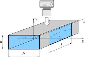
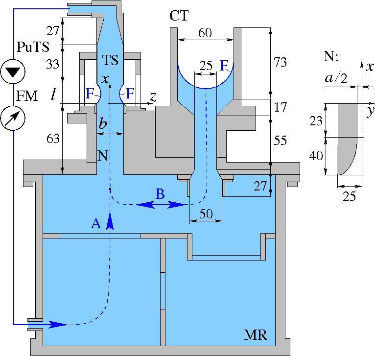
The main liquid loop is driven by a pump with a flow rate Q along streamline a (Figure 1, right) and through the channel (camera image). The secondary flow along streamline b is a consequence of surface movement and liquid displacement from the channel into the compensation tube and back.
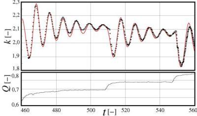
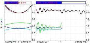
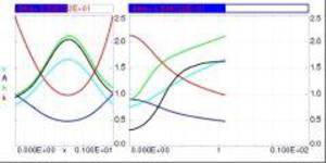
The dimensionless governing equations of the model are the unsteady momentum equation, the unsteady continuity equation and geometrical conditions of the channel and the surfaces. The unsteady model is verified by comparison to results of a sounding rocket experiment (TEXUS 41). The numerical solution of the model is in very good agreement to the observed oscillation of the liquid surface k (Figure 2). Furthermore, 3D computations confirm the assumed boundary conditions (see 3D video).
STABLE AND INSTABLE QUASI STEADY FLOW, 3D computation with OpenFOAM (click for video)
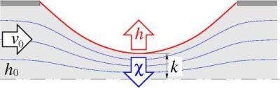
The surface stability is defined by the pressure interaction. In case of steady stable flow the capillary pressure h balances the flow induced convective pressure Χ (Figure 3). The surface position is k. The capillary pressure is based on the surface curvature and acts stabilazing. The convective pressure is mainly a function of the power of the flow velocity v2 and may cause system destabilization.
Increasing of the flow rate (in small steps) at the channel outlet generates longitudinal small capillary waves moving upstream (“flow rate increase signal"). At a critical flow rate the flow velocity v reaches the value of the wave velocity vca, “choking” occurs and the channel inlet and outlet are disconnected. This effect is related to the Speed Index Sca, which reaches at a critical point Sca=1, in analogy to the Mach Number.
In case of steady flow the surfaces collapse immediately at critical flow rate. Supercritical flow does not exist for steady flow and the critical flow rate represents the maximum stable value. Unsteady flow may be temporarily supercritical but remain stable. The unsteady effect is defined by the flow dynamic, which is the flow rate increase over time δ=ΔQ/Δt at the channel outlet. Increasing of the flow rate causes an increase of the pressure effects. The stability limit for unsteady flow is given by the ratio of the local capillary pressure and the local convective pressure, defining the Dynamic Index D. The free surfaces collapse at D=1.
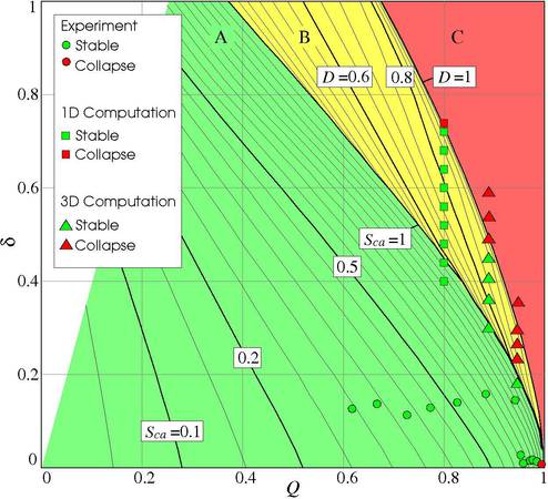
The result of this studies is a dynamic flow diagram (Figures 4 and 5) with the subcritical flow regime (green, Sca<1), the supercritical (choked) stable regime (yellow, Sca>1, D<1) and the limit of stable flow (D=1). For steady flow (δ=0) critical flow (Sca=1) is obviously equal to the stability limit of the system (D=1) so that supercritical steady flow is not possible.
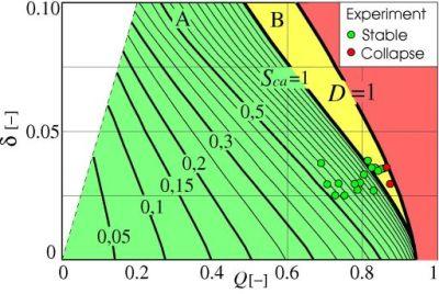
The unsteady maximum flow rate is smaller than for steady flow. On the other side, the choking effect does not necessarily cause surface collapse for unsteady flow and supercritical flow is temporarily possible. The dots represent stable (green) and unstable (red) flow rate dynamics, observed in the experiment. The unstable experimental dynamics match well to the theoretical stability limit of the system.